Indexes_

An index is a lookup structure the database maintains next to a table so it can find rows without scanning everything; the default B-tree kind keeps its entries sorted. Reads get faster; writes pay a small tax to keep each index current. Knowing when an index helps, and how to confirm it's being used, is the highest-leverage performance skill in SQL.

Setup

Index behavior only shows up with enough data on the table, so the setup seeds 100,000 users to give the query planner a real choice to make:

CREATE TABLE users (
    id         bigint GENERATED ALWAYS AS IDENTITY PRIMARY KEY,
    email      text NOT NULL,
    country    text NOT NULL,
    created_at timestamptz NOT NULL
);

INSERT INTO users (email, country, created_at)
SELECT 'user' || n || '@example.com',
       (ARRAY['DE','US','IN','BR'])[1 + n % 4],
       now() - (n || ' minutes')::interval
FROM generate_series(1, 100000) AS n;

ANALYZE users;

ANALYZE refreshes the statistics the planner uses to estimate row counts. PostgreSQL runs it automatically in the background; running it manually after a bulk load just avoids waiting.

How an index works

Table rows are stored in no order useful for searching an arbitrary column, so answering WHERE email = '...' without an index means reading every row and checking each one. The work grows with the table: ten times the rows, ten times the reads.

A B-tree (balanced tree) is the data structure indexes use to fix this. It keeps every value of the indexed column in sorted order, stored as a tree of small pages: the top page holds a few boundary values that direct the search into one of its child pages, each child narrows the range further, and the bottom layer, the leaves, holds the actual values with pointers back to their rows. Sorted order is what makes searching cheap:

• The database starts in the middle of the index, checks whether the target value sorts before or after that point, and discards the half that cannot contain it. Repeating this takes a handful of steps even on millions of rows.
• Equal values sit next to each other, so one descent lands on every matching entry at once.
• The same sorted order answers range conditions (<, BETWEEN) and returns rows already sorted for ORDER BY.

Indexes have a price: each one is a second copy of the column that must be kept correct, so every insert, update, and delete on the table also rewrites part of every index. They trade write work and disk space for read speed, which is why you add them for the queries you actually run rather than on every column.

Reading EXPLAIN ANALYZE

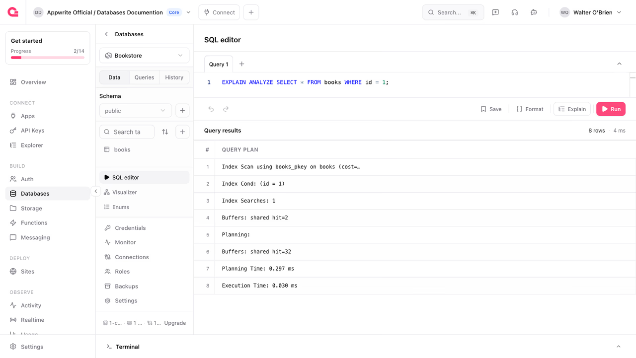
Before adding indexes, you need to see what the database is currently doing. Prefix any query with EXPLAIN ANALYZE and instead of returning its result, the database runs it and reports the plan it used:

EXPLAIN ANALYZE SELECT * FROM users WHERE email = 'user4242@example.com';

 Seq Scan on users  (cost=0.00..2175.00 rows=1 width=40) (actual time=0.141..2.565 rows=1.00 loops=1)
   Filter: (email = 'user4242@example.com'::text)
   Rows Removed by Filter: 99999

Reading it line by line:

• Seq Scan on users is the chosen strategy: a sequential scan, reading the table start to finish.
• Filter is the condition checked against every row as it's read.
• Rows Removed by Filter: 99999 is the waste: 100,000 rows read, 99,999 discarded, 1 returned.
• actual time=0.141..2.565 is when the first and last row were produced, in milliseconds. The cost numbers are the planner's internal estimates for comparing candidate plans, not milliseconds.

Exact numbers will differ on your database; the plan shape is what matters, and this shape, an entire table read to return one row, is the signal that an index would help. Plain EXPLAIN without ANALYZE shows the plan without executing the query, which is safer for slow queries and writes.

Create an index

CREATE INDEX builds the structure from the table's existing rows and keeps it maintained on every future write. Rerunning the earlier query shows the planner picking it up immediately:

CREATE INDEX idx_users_email ON users (email);

EXPLAIN ANALYZE SELECT * FROM users WHERE email = 'user4242@example.com';

 Index Scan using idx_users_email on users  (cost=0.42..8.44 rows=1 width=40) (actual time=0.019..0.019 rows=1.00 loops=1)
   Index Cond: (email = 'user4242@example.com'::text)

The plan flipped to an Index Scan, and execution time dropped from milliseconds to microseconds.

One B-tree index serves several kinds of conditions on its column:

• equality: = and IN
• ranges: <, >, BETWEEN
• sorting: ORDER BY
• prefix patterns like LIKE 'user42%', with a caveat: a normal index sorts text by human-language rules, which don't match how LIKE compares characters, so prefix searches ignore it. Adding the text_pattern_ops option when creating the index makes them work.

Primary keys and UNIQUE constraints create B-tree indexes automatically, so don't add duplicates for those columns.

Composite indexes and column order

An index on multiple columns is sorted by the first column, then the second within it, like a phone book sorted by last name, then first name. Column order decides which queries it serves:

CREATE INDEX idx_users_email_created ON users (email, created_at);

This index answers WHERE email = ..., and WHERE email = ... AND created_at > ..., but a filter on created_at alone can't use the sorted order because entries for every email are interleaved:

EXPLAIN SELECT * FROM users WHERE created_at > now() - interval '1 day';

 Seq Scan on users  (cost=0.00..2675.00 rows=1428 width=40)
   Filter: (created_at > (now() - '1 day'::interval))

Rule of thumb: put equality-filtered columns first and range-filtered columns last. If you also query created_at on its own, that's a separate index.

Covering indexes

A normal index lookup is two steps: find the matching entries in the index, then fetch each matching row from the table to read the other columns. That second step is the expensive part, and it's unnecessary when the query only asks for columns the index already stores.

This query selects only email, and the index contains email, so the answer comes straight out of the index:

EXPLAIN ANALYZE SELECT email FROM users WHERE email = 'user4242@example.com';

 Index Only Scan using idx_users_email_created on users  (cost=0.42..4.44 rows=1 width=21) (actual time=0.041..0.041 rows=1.00 loops=1)
   Index Cond: (email = 'user4242@example.com'::text)
   Heap Fetches: 0

• Index Only Scan is the plan node for answering from the index alone.
• Heap Fetches: 0 confirms the table was read zero times.

An index that satisfies a query this way is called a covering index. If a query also reads one extra column, you can add that column to the index with the INCLUDE option, which stores it alongside the entries without making it searchable.

Partial indexes

A partial index covers only rows matching a condition. It's smaller and cheaper to maintain than a full index, ideal when queries always target the same slice:

CREATE INDEX idx_users_recent_de ON users (created_at) WHERE country = 'DE';

The planner considers this index only for queries whose WHERE clause implies the index's condition, so include the country = 'DE' filter in queries that should use it. Common uses: unshipped orders, active sessions, rows where a nullable column is set.

Expression indexes

Indexing an expression makes queries on that expression fast, such as case-insensitive lookups:

CREATE INDEX idx_users_email_lower ON users (lower(email));

EXPLAIN SELECT * FROM users WHERE lower(email) = 'user4242@example.com';

 Bitmap Heap Scan on users  (cost=16.29..828.37 rows=500 width=40)
   Recheck Cond: (lower(email) = 'user4242@example.com'::text)
   ->  Bitmap Index Scan on idx_users_email_lower  (cost=0.00..16.17 rows=500 width=0)

The query's expression must match the indexed expression exactly. A Bitmap Index Scan is another index-driven strategy: PostgreSQL collects matching row locations from the index first, then fetches them from the table in physical order.

Beyond B-tree

PostgreSQL ships six index access methods. B-tree is the default and right for most columns; the others serve specific data shapes:

The cost of indexes

Every index consumes disk and slows every INSERT, UPDATE, and DELETE on the table, because each write updates each index. They add up quickly:

SELECT pg_size_pretty(pg_relation_size('users')) AS table_size,
       pg_size_pretty(pg_relation_size('idx_users_email')) AS index_size;

 table_size | index_size
------------+------------
 7400 kB    | 3992 kB

One index here costs more than half the table's size again. Index the queries you actually run, verify each index earns its keep with EXPLAIN, and drop the ones that don't. To find slow queries worth indexing in the first place, see Monitoring.